Understanding the amount of roadside space across a borough is invaluable for local authorities to implement effective and considered public realm schemes. Ranging from electric vehicle charging infrastructure allocation, supporting the transition to greener modes of transport, to social distancing measures ensuring the safety of residents and visitors. This blog outlines a method to compute the precise width of all pavements in Westminster using data from Ordnance Survey. The final map can be seen here

Credit: Joi Ito (CC BY 2.0)

Table of Contents

• Introduction

  • Motivation
  • Ordnance Survey
  • Data Cleaning

• Voronoi Tessalation

• Analysis

• Conclusions

• References

Introduction

Motivation

Although there are some examples of analysis being done to to calculate the pavement widths within a borough (for example), they usually are only sampling a small number of streets or categorising the streets into a few groups (e.g. <2m and >2m). The need for a higher precision could prove imperative for schemes such as:

• On street furnature allocation:
  • Electric Vehicles Charging Points
  • E-Scooters Docking Stations
  • TfL Public Bike Docking Stations
• Social Distancing Measure for Pandemic Planning
• Al Fresco Dining
• Ensuring accessability standards for everybody

Ordnance Survey

Data for this report comes from the Ordnance Survey API which can be accessed here. Specifically, the OS Features API was used with the custom filter to only extract the roadside polygons within the Westminster area. Because the roadside data is just a polygon layer, no information regarding the width (or in fact which road it belongs to) is included. This information will have to be derived. As well as pavement polygons, road lines will also be needed. Both datasets can be seen below:

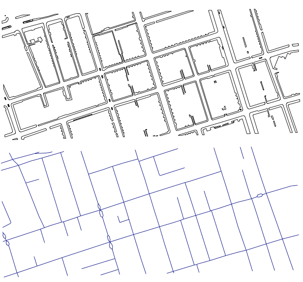
Figure 1: (Top): Roadside polygons returned from the Ordnance Survey API. (Bottom): Road lines returned from Ordnance Survey API

Data Cleaning

Before we can calculate the pavement widths for this dataset, a number of cleaning steps will need to be taked. Firstly, all internal boundaries need to be dissolved so the measurement we are taking is of the entire pavement and not just a section of it. Secondly, closely examining the data shows that it also contains the driveways and porches of the residential building adjacent to the road. These features can be seen in Figure 1 as the numerous square outcroppings along many of the roads. As these are not part of the public footway, they will need to be removed. To do this a custom algorithm can be applied to detect and remove these features from the data. This can be seen in the following figure:

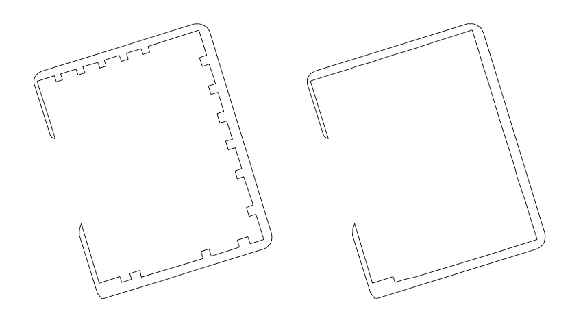
Figure 2: Data cleaning step. Driveways and residential porches removed to leave only the public pavement in the data.

Voronoi Tessalation

Voronoi tesselations crop up in a vast number of scientific disciplines. From boilogy, in the growth of the wings of a dragonfly (cover image at top), to material science when modelling the polycrystalline microscruture of metallic alloys. Hover your mouse over the image below to see how the voronoi tesseltions work:

These tessellations can easily be implemented in R with the sf package. The following code creates some random points and computes the voronoi tesselation.

library(sf)

# create 5 random points
x <- st_multipoint(matrix(runif(10),,2))

# compute and plot voronoi triangles
st_voronoi(x) %>% plot(col=0)

# plot original points
plot(x, add=T, col="darkblue", pch=19)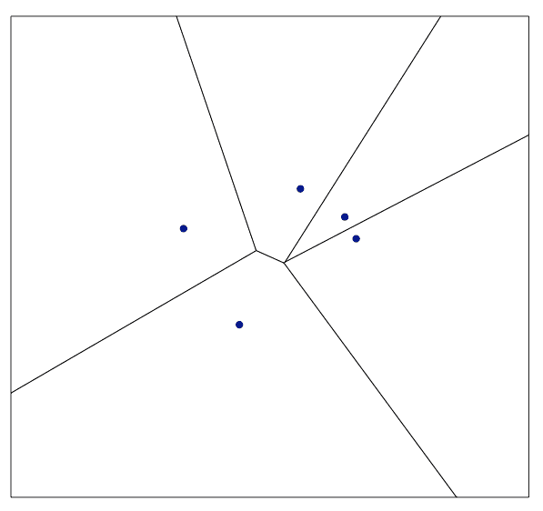

Voronoi tesselations can be applied to this analysis as well. As we do not know which pavements corespond to which road, we can segment the area around road and assign the pavements to the nearest road line. This seems to work to work surprisingly well as if a shape belong to multiple roads, it can be split up into multiple sections.

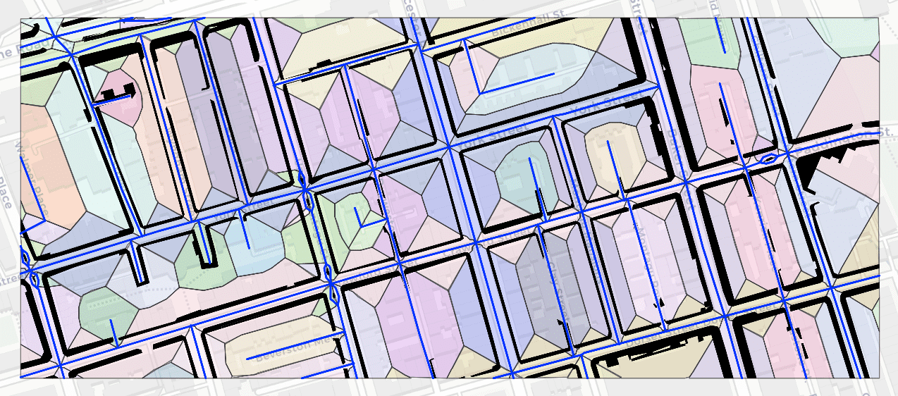
Figure 3: Voronoi tessalation to segment 'black' roadside polygons to the nearest 'blue' road line. The shaded polygons indicate the segmented area around each road line.

Following this step we now have a large array of pavement/road pairs like the image below.

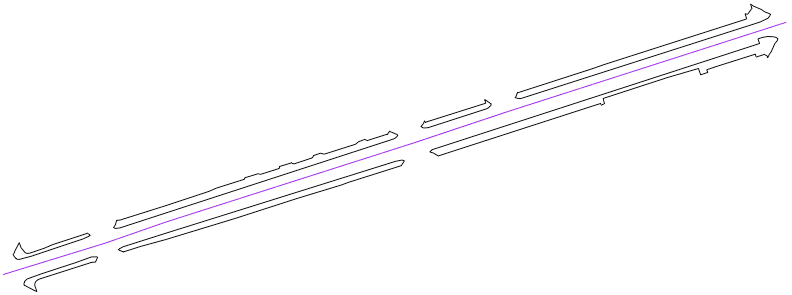
Figure 5: Road and Pavement.

Analysis

rot = function(a) matrix(c(cos(a), sin(a), -sin(a), cos(a)), 2, 2)

# Rotate rode segment using the rotation matrix with value of pi/2
rot(pi/2)

# Rotation Function
rot = function(a) matrix(c(cos(a), sin(a), -sin(a), cos(a)), 2, 2)

# Create line
line <- st_linestring(matrix(c( -2 , 2 , -4 , 4 ), 2, 2))
# Rotate line 90 degrees using the rotation matrix with value of pi/2
rotated_line <- line * rot(pi/2)

# Plot lines
plot(line)
plot(rotated_line, add=T, col="blue")

Figure 4: Rotation matrix appled to linestring

library(sf)

# roads - sf POLYLINES object of westminster roads
# crs - epsg:27700
roads_voronoi <- roads %>%
    st_line_sample(density=10) %>%
    st_union()
    st_voronoi()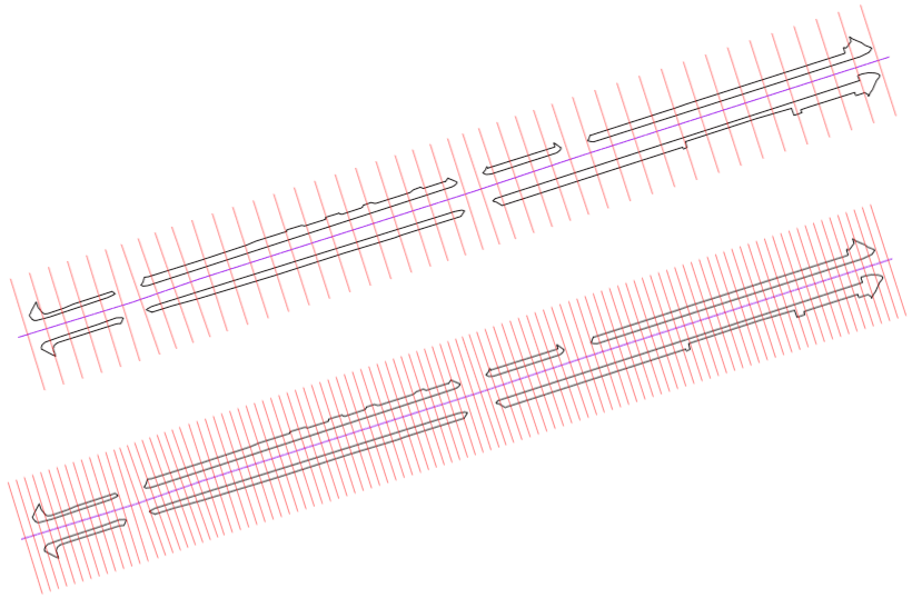

Figure 6: Frequency of perpendicular lines depending on precision required (red).

 # Calculate the width at regular intervals along the pavement 
 # by intersecting the perpendiuclar lines with the roadside polygons
 pavement_widths <- perpendicular_lines %>%
    st_intersection(roadside)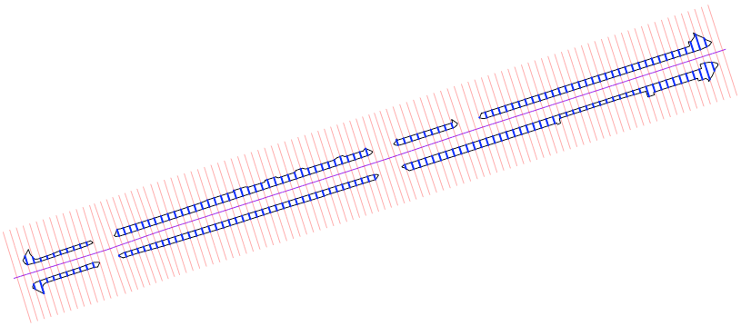 

Figure 7: Intersection with the pavement to determine width at that point (blue).

Conclusions

References